import spaceprime as spspaceprime for R users
Introduction
The primary reason for implementing spaceprime in Python is to facilitate a natural integration with the msprime library. While there are R packages that can interface with msprime, most notably slendr, maintaining the connection between R and Python adds significant maintenance overhead. If someone wants to pay me to maintain it, I’d be happy to create an R API, but until then, Python it is! It’s also good to learn a little Python- it’s a very useful language to know. Fortunately, you don’t have to be an expert in Python to use spaceprime, so I’ll get you up to speed on the basics.
Installation
In R, package installation is designed to be easy, which is manageable due to R’s limited scope. Python is an incredibly diverse language, so flexibility in package design and management is valued more than ease of use. The focus then is to create unique development environments for the projects you are working on. This facilitates reproducibility as well as an explicit and clean developing environment.
To maintain a clean developing environment, it’s common practice to use a virtual environment for your projects. This is a self-contained Python environment that allows you to install packages without affecting your system Python installation. The most popular package for managing virtual environments is conda. There are multiple conda distributions, but I recommend installing the miniforge distribution, which contains the mamba package manager. Mamba is a faster, more efficient package manager than conda, and it’s what I use to install packages. If you’re already familiar with conda, mamba is a drop-in replacement.
Once you have miniforge installed, you can create a new environment with the following command:
mamba create -n spaceprimeThis will create a new environment called spaceprime. To activate the environment, use the following command:
mamba activate spaceprimeNow, when you install packages, they will be installed in the spaceprime environment. To install the packages you need for this tutorial, use the following command:
mamba install spaceprime rasterio geopandasThe rasterio and geopandas packages are used for reading in and manipulating spatial data. I’ll discuss them in more detail later.
Loading packages
In Python, you load packages using the import statement. For example, to load the spaceprime package, you would use the following command:
The as sp part of the command is an alias, which allows you to refer to the package by a shorter name. You want to do this for longer package names to save typing. Python requires you to use the package name when calling functions from the package, rather than it being optional, like in R. For example, to call a function from the spaceprime package, you would use the following syntax:
sp.function_name()This is analogous to the package::function_name() syntax in R.
In Python, you can also import specific modules or functions from a package, rather than importing the entire package. For example, to import just the demography module from the spaceprime package, you would use the following command:
from spaceprime import demography
TipModules
In Python, a module is a file that contains code you can use to perform specific tasks. This code can include functions, variables, and classes. Python packages typically contain multiple modules, each of which performs a specific set of tasks. Unlike in R, Python allows you to import specific modules or functions from a package, rather than having to load the entire package.
If you want to just import the raster_to_demes() function from the utilities module, you would use the following command:
from spaceprime.utilities import raster_to_demesImport the necessary packages
For this tutorial, we’ll be using the spaceprime, rasterio, and geopandas packages.
import spaceprime as sp
import rasterio
import geopandas as gpd
The rasterio package is used for reading, manipulating, and writing raster data, with its closest R analogue being the terra package. The geopandas package is used for reading, manipulating, and writing vector data, with its closest R analogue being the sf package.
Download data
The data we’re using in this example are a GeoTiff raster file of habitat suitability values and a GeoJSON file containing geographic localities and metadata for this cute frog, Phyllomedusa distincta:

Follow the link to download the projections.tif file. You do not need to download the localities.geojson file, as it is read in from the web in the code below.
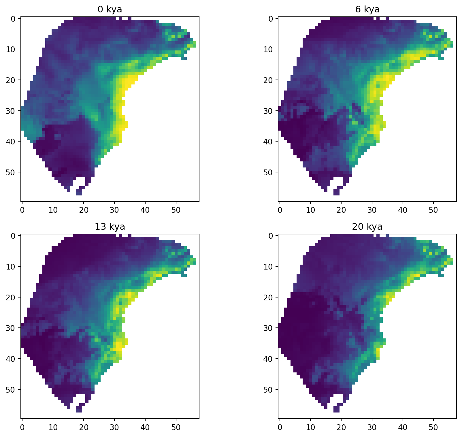
The raster file contains 23 layers, where each layer is a projection of the habitat suitability model (aka species distribution model or ecological niche model) to a time slice in the past, ranging from the present day to 22,000 years ago in 1,000 year intervals. The habitat suitability values range from zero to one, where zero represents no suitability for the species and one represents perfect suitability. In the following plots, yellow represents higher suitability and purple represents lower suitability. Here are a few time slices of the model:
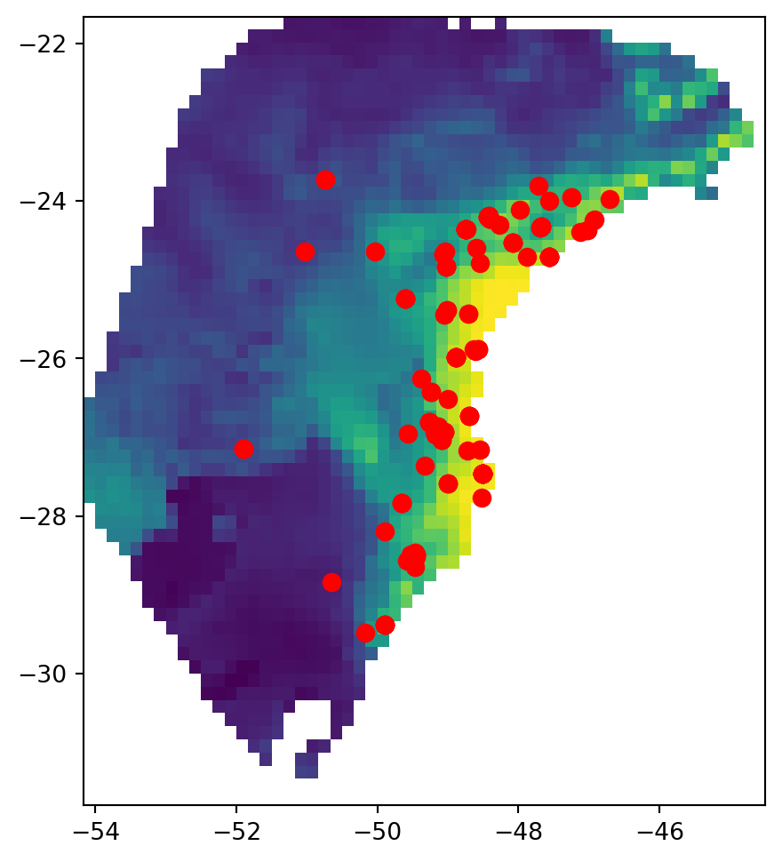
The GeoJSON file contains geographic sampling localities of P. distincta in the Brazilian Atlantic Forest, along with metadata about each locality. Each row is a single individual/observation. spaceprime counts the number of observations with coordinates that overlap with a raster cell/deme and samples the calculated number for simulations and summary statistics. Here are the localities plotted on top of the present-day habitat suitability model:
Read in data
Make sure to replace the projections.tif file path with the path to the file on your system. The GeoJSON file is read in from the web, so you don’t need to download it. Notice that each function is called with the package name or alias followed by a period, then the function name!
r = rasterio.open("projections.tif")
locs = gpd.read_file("https://raw.githubusercontent.com/connor-french/spaceprime/main/spaceprime/data/localities.geojson")
To check out your raster object, you can print the meta attribute to the console. This will give you a summary of the raster, including the number of bands, the width and height of the raster, the coordinate reference system (CRS), and the bounds of the raster.
print(r.meta){'driver': 'GTiff', 'dtype': 'float32', 'nodata': nan, 'width': 58, 'height': 60, 'count': 23, 'crs': CRS.from_wkt('GEOGCS["WGS 84",DATUM["WGS_1984",SPHEROID["WGS 84",6378137,298.257223563,AUTHORITY["EPSG","7030"]],AUTHORITY["EPSG","6326"]],PRIMEM["Greenwich",0,AUTHORITY["EPSG","8901"]],UNIT["degree",0.0174532925199433,AUTHORITY["EPSG","9122"]],AXIS["Latitude",NORTH],AXIS["Longitude",EAST],AUTHORITY["EPSG","4326"]]'), 'transform': Affine(0.16666666600000002, 0.0, -54.16680605885,
0.0, -0.166666666, -21.666805828849988)}To check out your GeoDataFrame object, use the head() method, which will print the first few rows to your console.
locs.head()| species | longitude | latitude | individual_id | anc_pop_id | geometry | |
|---|---|---|---|---|---|---|
| 0 | distincta | -48.633300 | -25.883300 | 1145545021 | 1.0 | POINT (-48.6333 -25.8833) |
| 1 | distincta | -48.716829 | -27.169879 | 3044567206 | 2.0 | POINT (-48.71683 -27.16988) |
| 2 | distincta | -47.983204 | -24.116604 | 2596355434 | 1.0 | POINT (-47.9832 -24.1166) |
| 3 | distincta | -47.014321 | -24.369859 | 3772589489 | 1.0 | POINT (-47.01432 -24.36986) |
| 4 | distincta | -49.581356 | -28.559573 | 2448001684 | 2.0 | POINT (-49.58136 -28.55957) |
If you would like to perform further data exploration on your GeoDataFrame object, I highly recommend the plotnine package, which is a Python implementation of the ggplot2 package in R. It uses the grammar of graphics to make nice plots. It’s the most painless way to switch from R plotting to Python plotting.
Set up the demographic model
Next, we’ll convert the habitat suitability values into deme sizes, so each cell in the raster will represent a deme in our model. We’ll use a linear transformation to convert the suitability values to deme sizes, where the suitability value is multiplied by a constant to get the deme size. The constant is the maximum local deme size, which we set to 1000. For more on transformations, see the suitability to deme size transformation functions vignette.
d = sp.raster_to_demes(r, transformation="linear", max_local_size=1000)Now that we have our deme sizes, we can set up the demographic model. spaceprime uses an object-oriented programming paradigm for creating a demographic model. Although most R users are more familiar with a functional programming paradigm, object-oriented programming does exist in R.
In object-oriented programming, you create an instance of a class and then call methods on that instance. The class is like a blueprint for creating objects, and the methods are functions that operate on the object’s data. This is useful for creating complex data structures like demographic models, where you have multiple components that interact with each other.
In spaceprime, the spDemography class is used to set up the demographic model. The spDemography class has methods for setting up the spatial component of the model, adding ancestral populations, and inherits all of the methods of the msprime Demography class.
demo = sp.spDemography()Now you can run methods on the demo object to set up the demographic model. The first method we’ll run is the stepping_stone_2d() method, which sets up a two-dimensional stepping-stone model. The migration rate, specified by rate, can be a single global rate or an array of values specifying each neighbor’s migration rate. Here, we’re using a global rate of 0.001. The global rate by default is scaled, where demes exchange the same number of migrants with their neighbors, regardless of deme size. To change this behavior, set scale=false. We’re assuming that P. distincta has a generation time of one year. Using a single value for the timesteps argument tells spaceprime that 1000 generations passes in between each raster time step in the model.
This step may take a few seconds (10-15 seconds on my machine) to run.
# populate the spDemography object with the deme sizes and migration rates
demo.stepping_stone_2d(d, rate=0.001, timesteps=1000)
You may have noticed that we didn’t assign the output to a new variable. This is because the stepping_stone_2d() method modifies the demo object in place, rather than returning a new object. This is a common pattern in object-oriented programming, where methods modify the object they’re called on rather than returning a new object.
After initializing the spatial component of the simulation, it’s desirable to add one or more ancestral populations to the model. This is done by providing a list of ancestral population sizes and the time (in generations) at which the spatially distributed demes migrate into the ancestral population(s). The following code adds a single ancestral population of 100,000 individuals that demes merge into 23,000 generations in the past. The brackets in [100000] specify a list in python. In this case, it is a list of length one.
# add ancestral population
demo.add_ancestral_populations([100000], 23000)
Inspect your model
Now that we have our demographic model set up, we can inspect it to make sure it looks as expected. spaceprime has a series of plot_() functions that make this easier.
plot_landscape()
plot_landscape() plots the deme sizes in space, which allows you to quickly inspect whether the transformation you applied to your habitat suitability map make sense. Here, we provide the demographic model object, the raster object, the index of the time slice to plot (0 for the present day in this case), and basemap=True to add an OpenStreetMap basemap, providing geographic context to the plot. If you don’t have an internet connection, set basemap=False (the default) to plot without the basemap.
sp.plot_landscape(demo, r, 0, basemap=True)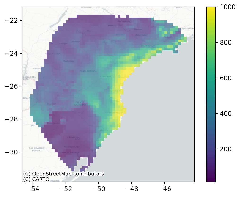
plot_model()
plot_model() plots the deme sizes on a folium interactive map, with precise deme sizes and outgoing migration rates for each deme present in a popup.
sp.plot_model(demo, r, 0)Make this Notebook Trusted to load map: File -> Trust Notebook
Simulate genetic data
Before simulating this demography, we need to create a sample dictionary that translates the empirical sampling localities to the model’s deme indices and maps those to the number of samples to take from each deme. By default, coords_to_sample_dict() sets the number of individuals to sample from each deme to the number of empirical localities in that deme. The function also returns two other dictionaries that are not used in this example, so we’ll ignore them. In Python, it’s common practice for a function to return multiple objects as a list. If you want the objects separated, you use the formatting below. Using an underscore _ leads to the object being ignored.
NoteDictionaries
Dictionaries are a data structure in Python that map keys to values. They are similar to lists, but instead of using an index to access elements, you use a key. Dictionaries are useful for storing data that has a key-value relationship, like a phone book, where the key is the name of the person and the value is their phone number. In this case, the key is the deme index and the value is the number of samples to take from that deme.
sample_dict, _, _ = sp.coords_to_sample_dict(r, locs)Now we get to simulate! The first task is to simulate the ancestry of the samples using the coalescent. All of the hard work is done through msprime’s sim_ancestry() function, for which spaceprime provides a convenience wrapper. This function returns a tskit TreeSequence, which “represents a sequence of correlated evolutionary trees along a genome” and is an incredibly powerful and compact data representation for population genomic analyses. The minimum number of arguments required for this function are the sample dictionary and the demographic model. If you need to overlay mutations, you need to supply the sequence length. Notice the lack of mutations in the table. We’ll set record_provenance to False to decrease the memory overhead of storing a bunch of metadata about the simulation.
This step may take a minute or so to run.
sim = sp.sim_ancestry(samples=sample_dict, demography=demo, sequence_length=1e5, record_provenance=False, random_seed=42)

print(sim)
╔═══════════════════════════╗
║TreeSequence ║
╠═══════════════╤═══════════╣
║Trees │ 1║
╟───────────────┼───────────╢
║Sequence Length│ 100,000║
╟───────────────┼───────────╢
║Time Units │generations║
╟───────────────┼───────────╢
║Sample Nodes │ 344║
╟───────────────┼───────────╢
║Total Size │ 205.8 KiB║
╚═══════════════╧═══════════╝
╔═══════════╤═════╤═════════╤════════════╗
║Table │Rows │Size │Has Metadata║
╠═══════════╪═════╪═════════╪════════════╣
║Edges │ 686│ 21.4 KiB│ No║
╟───────────┼─────┼─────────┼────────────╢
║Individuals│ 172│ 4.7 KiB│ No║
╟───────────┼─────┼─────────┼────────────╢
║Migrations │ 0│ 8 Bytes│ No║
╟───────────┼─────┼─────────┼────────────╢
║Mutations │ 0│ 16 Bytes│ No║
╟───────────┼─────┼─────────┼────────────╢
║Nodes │ 687│ 18.8 KiB│ No║
╟───────────┼─────┼─────────┼────────────╢
║Populations│3,481│155.4 KiB│ Yes║
╟───────────┼─────┼─────────┼────────────╢
║Provenances│ 0│ 16 Bytes│ No║
╟───────────┼─────┼─────────┼────────────╢
║Sites │ 0│ 16 Bytes│ No║
╚═══════════╧═════╧═════════╧════════════╝
We’ll take a peak at a single tree from the TreeSequence object to see what it looks like. The draw_svg() method plots trees from the TreeSequence object. Here, I selected a single tree and removed the node labels because there are tons of nodes that crowd the plot and we’re only interested in the tree structure.
first_tree = sim.first()
node_labels = {node.id: "" for node in sim.nodes()}
first_tree.draw_svg(y_axis=True, size=(600, 400), node_labels=node_labels)
Overlaying mutations after simulating ancestry isn’t necessary for calculating genetic summary statistics on a TreeSequence, but it is necessary if you would like to compare your simulations with empirical data that are represented as a table of genotypes rather than a TreeSequence. The sim_mutations() function overlays mutations on the TreeSequence object returned by sim_ancestry() and requires the mutation rate. The mutation rate is the number of mutations per base pair per generation. For this example, we’ll use a mutation rate of 1e-10 so we don’t overcrowd the tree sequence visualization. You can see from the table that the tree sequence has some mutations!
sim = sp.sim_mutations(sim, rate=1e-10, random_seed=490)

print(sim)
╔═══════════════════════════╗
║TreeSequence ║
╠═══════════════╤═══════════╣
║Trees │ 1║
╟───────────────┼───────────╢
║Sequence Length│ 100,000║
╟───────────────┼───────────╢
║Time Units │generations║
╟───────────────┼───────────╢
║Sample Nodes │ 344║
╟───────────────┼───────────╢
║Total Size │ 209.4 KiB║
╚═══════════════╧═══════════╝
╔═══════════╤═════╤═════════╤════════════╗
║Table │Rows │Size │Has Metadata║
╠═══════════╪═════╪═════════╪════════════╣
║Edges │ 686│ 21.4 KiB│ No║
╟───────────┼─────┼─────────┼────────────╢
║Individuals│ 172│ 4.7 KiB│ No║
╟───────────┼─────┼─────────┼────────────╢
║Migrations │ 0│ 8 Bytes│ No║
╟───────────┼─────┼─────────┼────────────╢
║Mutations │ 48│ 1.8 KiB│ No║
╟───────────┼─────┼─────────┼────────────╢
║Nodes │ 687│ 18.8 KiB│ No║
╟───────────┼─────┼─────────┼────────────╢
║Populations│3,481│155.4 KiB│ Yes║
╟───────────┼─────┼─────────┼────────────╢
║Provenances│ 1│719 Bytes│ No║
╟───────────┼─────┼─────────┼────────────╢
║Sites │ 48│ 1.2 KiB│ No║
╚═══════════╧═════╧═════════╧════════════╝
You might have noticed that we return new objects for sim_ancestry and sim_mutations. This is because we have returned to a functional programming paradigm, where functions return new objects rather than modifying objects in place. We do this because the TreeSequence objects are a different type of object than the demographic model object, and we want to keep them separate.
And now for the tree. The red X’s represent mutations on the tree, with their ID numbers next to them.
first_tree_mut = sim.first()

node_labels = {node.id: "" for node in sim.nodes()}
first_tree_mut.draw_svg(y_axis=True, size=(600, 400), node_labels=node_labels)
From here, you have a few options. You can:
- Use the
analysismodule to calculate genetic summary statistics on the TreeSequence object. For more on theanalysismodule, see the analysis module documentation.
- Save the TreeSequence to use later or analyze on a platform like tskit with
sim.dump(file/path/to/write/to.trees).
- Convert the TreeSequence with mutations to a genotype matrix for use in a program like scikit-allel with
sim.genotype_matrix(). For more information on this function, see the tskit documentation.
- Export the TreeSequence with mutations to a VCF file using
sim.write_vcf. For more information on how to use this function, see the tskit documentation.
WarningTODO
add a link to the analysis module documentation when it’s ready.