spaceprime

A python package to facilitate spatially explicit coalescent modeling in msprime

• Free software: MIT License
• Documentation: https://connor-french.github.io/spaceprime

Overview

spaceprime is a Python package that facilitates the creation and analysis of spatially gridded coalescent models in the msprime library. The package is designed to make it easier for practitioners to convert spatial maps of habitat suitability into extensible two-dimensional stepping-stone models of gene flow, where each pixel of the map represents a deme and demes are able to migrate with their neighbors. Demes and migration rates are able to change over time according to habitat suitability model projections to different time periods. These demographic parameters are then used to simulate genetic data under a coalescent model with msprime as the simulator, which can be used to infer the demographic history of the population. The package is designed to be user-friendly and intuitive, allowing users to easily simulate and analyze spatially explicit genetic data.

Note for R users

spaceprime is implemented in Python, yet many interested users may come from an R background. I have a spaceprime for R users vignette that provides a brief introduction to the Python concepts necessary to use spaceprime through a practical walk-through of an example analysis. If you still want to use R, it is possible to use Python code in R using the reticulate package. For more information on how to use Python code in R, see the reticulate documentation.

Main features

spaceprime includes a number of features:

• Convert habitat suitability values into demographic parameters, including deme sizes, migration rates, and their change through time using very little code. Code complexity does not increase with model complexity, allowing users to focus on the biological questions they are interested in.
  
• Simulate spatially explicit genetic data under a coalescent model with msprime. The modeling approach is fully coalescent with no forward-time component, allowing for computationally efficient simulations of large spatially explicit models.
  
• Visualize demographic models to facilitate model interpretation and model checking.
• Compute genetic summary statistics for simulated and empirical data to facilitate comparison with empirical data.
  
• Extensibility: spaceprime is designed to be interoperable with msprime, where users can setup a model with spaceprime, then customize it using the full range of msprime functionality.

Installation

Stable release

spaceprime can be installed using pip or conda. Due to the package’s reliance on msprime, the pip installation is only available on unix-based systems (MacOS, Linux). Windows users should install spaceprime using conda.

To install spaceprime using pip, run the following command in your terminal:

pip install spaceprime

To install spaceprime using conda, run the following command in your terminal:

conda install -c conda-forge spaceprime

The mamba package manager can also be used to install spaceprime using conda. mamba tends to be much faster than conda. To install spaceprime using mamba, install mamba, then run the following command in your terminal:

mamba install -c conda-forge spaceprime

From source

To install spaceprime from source, run this command in your terminal:

pip install git+https://github.com/connor-french/spaceprime

Extras

To install the analysis module, which is imported separately from the main package to reduce the number of dependencies:

pip install spaceprime[analysis]

or

conda install -c conda-forge spaceprime[analysis]

Usage

To use spaceprime in a project:

import spaceprime

To use the analysis module, which is imported separately from the main package to reduce the number of dependencies:

from spaceprime import analysis

Important

Make sure to install the relevant analysis dependencies with pip install spaceprime[analysis] or conda install -c conda-forge spaceprime[analysis].

Quickstart

Tip

This quickstart guide assumes you have a basic understanding of Python. If you are an R user, please refer to the spaceprime for R users vignette for an overview of spaceprime with the necessary Python concepts explained.

1. Download data

The data we’re using in this example are a GeoTiff raster file of habitat suitability values and a GeoJSON file containing geographic localities and metadata for this cute frog, Phyllomedusa distincta:

Follow the link to download the projections.tif file. You do not need to download the localities.geojson file, as it is read in from the web in the code below.

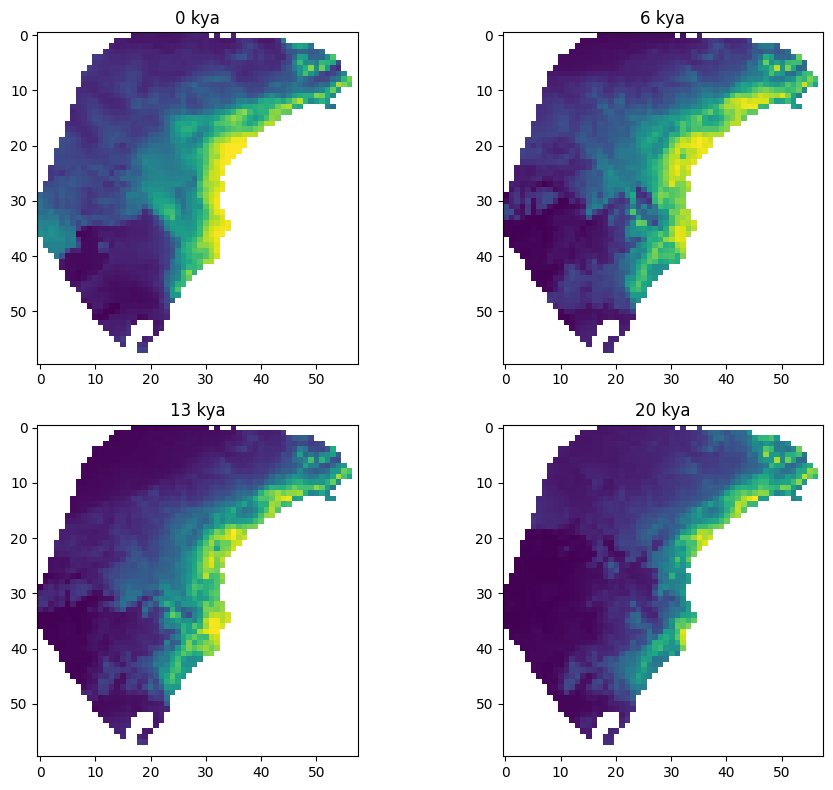
The raster file contains 23 layers, where each layer is a projection of the habitat suitability model (aka species distribution model or ecological niche model) to a time slice in the past, ranging from the present day to 22,000 years ago in 1,000 year intervals. The habitat suitability values range from zero to one, where zero represents no suitability for the species and one represents perfect suitability. In the following plots, yellow represents higher suitability and purple represents lower suitability. Here are a few time slices of the model:

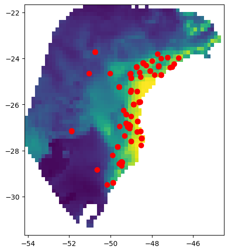
The GeoJSON file contains geographic sampling localities of P. distincta in the Brazilian Atlantic Forest, along with metadata about each locality. Each row is a single individual/observation. spaceprime counts the number of observations with coordinates that overlap with a raster cell/deme and samples the calculated number for simulations and summary statistics. Here are the localities plotted on top of the present-day habitat suitability model:

2. Read in packages and data

Now that we have our data, let’s read in the packages and data we’ll be using. The GeoPandas and Rasterio packages are dependencies of spaceprime, so you shouldn’t need to install them separately. They are needed for reading in locality data and habitat suitability rasters, respectively.

import spaceprime as sp
import geopandas as gpd
import rasterio

Make sure to replace the projections.tif file path with the path to the file on your system. The GeoJSON file is read in from the web, so you don’t need to download it.

r = rasterio.open("projections.tif")
locs = gpd.read_file("https://raw.githubusercontent.com/connor-french/spaceprime/main/spaceprime/data/localities.geojson")

3. Set up the demographic model

Next, we’ll convert the habitat suitability values into deme sizes, so each cell in the raster will represent a deme in our model. We’ll use a linear transformation to convert the suitability values to deme sizes, where the suitability value is multiplied by a constant to get the deme size. The constant is the maximum local deme size, which we set to 1000. For more on transformations, see the suitability to deme size transformation functions vignette.

d = sp.raster_to_demes(r, transformation="linear", max_local_size=1000)

Now that we have our deme sizes, we can set up the demographic model. The model that spaceprime uses is a two-dimensional stepping-stone model with a global migration rate of 0.001 between neighboring demes. The global rate by default is scaled, where demes exchange the same number of migrants with their neighbors, regardless of deme size. To change this behavior, set scale=false. We’re assuming that P. distincta has a generation time of one year. Using a single value for the timesteps argument tells spaceprime that 1000 generations passes in between each raster time step in the model.

This step may take a few seconds (10-15 seconds on my machine) to run.

# initialize the model
demo = sp.spDemography()

# populate the spDemography object with the deme sizes and migration rates
demo.stepping_stone_2d(d, rate=0.001, timesteps=1000)

After initializing the spatial component of the simulation, it’s desirable to add one or more ancestral populations to the model. This is done by providing a list of ancestral population sizes and the time (in generations) at which the spatially distributed demes migrate into the ancestral population(s). The following code adds a single ancestral population of 100,000 individuals that demes merge into 23,000 generations in the past:

# add ancestral population
demo.add_ancestral_populations([100000], 23000)

4. Inspect your model

Now that we have our demographic model set up, we can inspect it to make sure it looks as expected. spaceprime has a series of plot_() functions that make this easier.

plot_landscape()

plot_landscape() plots the deme sizes in space, which allows you to quickly inspect whether the transformation you applied to your habitat suitability map make sense. Here, we provide the demographic model object, the raster object, the index of the time slice to plot (0 for the present day in this case), and basemap=True to add an OpenStreetMap basemap, providing geographic context to the plot. If you don’t have an internet connection, set basemap=False (the default) to plot without the basemap.

sp.plot_landscape(demo, r, 0, basemap=True)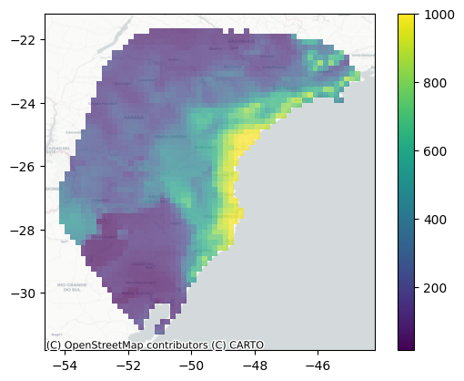

plot_model()

plot_model() plots the deme sizes on a folium interactive map, with precise deme sizes and outgoing migration rates for each deme present in a popup.

sp.plot_model(demo, r, 0)

Make this Notebook Trusted to load map: File -> Trust Notebook

5. Simulate genetic data

Before simulating this demography, we need to create a sample dictionary that translates the empirical sampling localities to the model’s deme indices and maps those to the number of samples to take from each deme. By default, this function sets the number of individuals to sample from each deme to the number of empirical localities in that deme. The coords_to_sample_dict() function also returns two other dictionaries that are not used in this example, so we’ll ignore them.

sample_dict, _, _ = sp.coords_to_sample_dict(r, locs)

Now we get to simulate! The first task is to simulate the ancestry of the samples using the coalescent. All of the hard work is done through msprime’s sim_ancestry() function, for which spaceprime provides a convenience wrapper. This function returns a tskit TreeSequence, which “represents a sequence of correlated evolutionary trees along a genome” and is an incredibly powerful and compact data representation for population genomic analyses. The minimum number of arguments required for this function are the sample dictionary and the demographic model. If you need to overlay mutations, you need to supply the sequence length. Notice the lack of mutations in the table. We’ll set record_provenance to False to decrease the memory overhead of storing a bunch of metadata about the simulation.

This step may take a minute or so to run.

sim = sp.sim_ancestry(samples=sample_dict, demography=demo, sequence_length=1e5, record_provenance=False, random_seed=42)

print(sim)

╔═══════════════════════════╗
║TreeSequence               ║
╠═══════════════╤═══════════╣
║Trees          │          1║
╟───────────────┼───────────╢
║Sequence Length│     100000║
╟───────────────┼───────────╢
║Time Units     │generations║
╟───────────────┼───────────╢
║Sample Nodes   │        344║
╟───────────────┼───────────╢
║Total Size     │  205.8 KiB║
╚═══════════════╧═══════════╝
╔═══════════╤════╤═════════╤════════════╗
║Table      │Rows│Size     │Has Metadata║
╠═══════════╪════╪═════════╪════════════╣
║Edges      │ 686│ 21.4 KiB│          No║
╟───────────┼────┼─────────┼────────────╢
║Individuals│ 172│  4.7 KiB│          No║
╟───────────┼────┼─────────┼────────────╢
║Migrations │   0│  8 Bytes│          No║
╟───────────┼────┼─────────┼────────────╢
║Mutations  │   0│ 16 Bytes│          No║
╟───────────┼────┼─────────┼────────────╢
║Nodes      │ 687│ 18.8 KiB│          No║
╟───────────┼────┼─────────┼────────────╢
║Populations│3481│155.4 KiB│         Yes║
╟───────────┼────┼─────────┼────────────╢
║Provenances│   0│ 16 Bytes│          No║
╟───────────┼────┼─────────┼────────────╢
║Sites      │   0│ 16 Bytes│          No║
╚═══════════╧════╧═════════╧════════════╝

We’ll take a peak at a single tree from the TreeSequence object to see what it looks like. The draw_svg() method plots trees from the TreeSequence object. Here, I selected a single tree and removed the node labels because there are tons of nodes that crowd the plot and we’re only interested in the tree structure.

first_tree = sim.first()
node_labels = {node.id: "" for node in sim.nodes()}
first_tree.draw_svg(y_axis=True, size=(600, 400), node_labels=node_labels)

Overlaying mutations after simulating ancestry isn’t necessary for calculating genetic summary statistics on a TreeSequence, but it is necessary if you would like to compare your simulations with empirical data that are represented as a table of genotypes rather than a TreeSequence. The sim_mutations() function overlays mutations on the TreeSequence object returned by sim_ancestry() and requires the mutation rate. The mutation rate is the number of mutations per base pair per generation. For this example, we’ll use a mutation rate of 1e-10 so we don’t overcrowd the tree sequence visualization. You can see from the table that the tree sequence has some mutations!

sim = sp.sim_mutations(sim, rate=1e-10, random_seed=490)

print(sim)

╔═══════════════════════════╗
║TreeSequence               ║
╠═══════════════╤═══════════╣
║Trees          │          1║
╟───────────────┼───────────╢
║Sequence Length│     100000║
╟───────────────┼───────────╢
║Time Units     │generations║
╟───────────────┼───────────╢
║Sample Nodes   │        344║
╟───────────────┼───────────╢
║Total Size     │  209.4 KiB║
╚═══════════════╧═══════════╝
╔═══════════╤════╤═════════╤════════════╗
║Table      │Rows│Size     │Has Metadata║
╠═══════════╪════╪═════════╪════════════╣
║Edges      │ 686│ 21.4 KiB│          No║
╟───────────┼────┼─────────┼────────────╢
║Individuals│ 172│  4.7 KiB│          No║
╟───────────┼────┼─────────┼────────────╢
║Migrations │   0│  8 Bytes│          No║
╟───────────┼────┼─────────┼────────────╢
║Mutations  │  48│  1.8 KiB│          No║
╟───────────┼────┼─────────┼────────────╢
║Nodes      │ 687│ 18.8 KiB│          No║
╟───────────┼────┼─────────┼────────────╢
║Populations│3481│155.4 KiB│         Yes║
╟───────────┼────┼─────────┼────────────╢
║Provenances│   1│716 Bytes│          No║
╟───────────┼────┼─────────┼────────────╢
║Sites      │  48│  1.2 KiB│          No║
╚═══════════╧════╧═════════╧════════════╝

And now for the tree. The red X’s represent mutations on the tree, with their ID numbers next to them.

first_tree_mut = sim.first()

node_labels = {node.id: "" for node in sim.nodes()}
first_tree_mut.draw_svg(y_axis=True, size=(600, 400), node_labels=node_labels)

From here, you have a few options. You can:

• Use the analysis module to calculate genetic summary statistics on the TreeSequence object. For more on the analysis module, see the analysis module documentation.
  
• Save the TreeSequence to use later or analyze on a platform like tskit with sim.dump(file/path/to/write/to.trees).
  
• Convert the TreeSequence with mutations to a genotype matrix for use in a program like scikit-allel with sim.genotype_matrix(). For more information on this function, see the tskit documentation.
  
• Export the TreeSequence with mutations to a VCF file using sim.write_vcf. For more information on how to use this function, see the tskit documentation.

TODO

add a link to the analysis module documentation when it’s ready.

Report Issues

https://github.com/connor-french/spaceprime/issues

Contributing

We love contributions! Please see the Contributing Guide for more information.

Please note that this project is released with a Contributor Code of Conduct. By participating in this project you agree to abide by its terms.